7 Microsoft Excel secrets for better spreadsheets

When creating a spreadsheet, you want to get the job done fast and create something effective, smart and professional looking. Our expert Microsoft Excel tips will help you do just that!
Let’s face it; spreadsheets aren’t exactly the most glamorous part of your working day. And very few people could say they have mastered everything the world’s most popular spreadsheet tool has to offer. Yet spreadsheets are often integral to most businesses and can form the basis of some big business decisions.
Microsoft Excel has an estimated 750 million to 1.2 billion monthly users globally and is considered by the company as their most important consumer product.
Source: The New Stack
What if your spreadsheets could work smarter, look smarter, and help you make smarter decisions? What if you could spend less time building your spreadsheets? Imagine how much time and energy you could save working with data in Excel if you knew the right shortcuts and tips to get there faster.
In this article, we reveal seven Excel secrets to help you create better spreadsheets with ease and in less time. But, of course, once you have read this article, they aren’t secrets anymore – just top tips you can share (or keep to yourself)!
Secret #1: Customise the Quick Access Toolbar
At the top left of Excel, you’ll see a cluster of small icons next to the Autosave function. This is a collection of shortcuts that you can customise to include your most frequently used actions.

These actions will be ever-present at the top of the screen. This is handy when you spend a lot of time moving between different tabs when in Excel (for example, between Home, Data, and Formulas).
Like many people, sorting columns of data is something we do a lot here at iHTTP, so we add the Sort Ascending and Sort Descending actions to our Quick Access Toolbar.

Dive into the full array of actions/commands available using the More Commands option. Here you can browse the most popular commands or search for the most common Excel features you use.
So we’re starting with quite a simple tip, but you would be surprised at how many regular Excel users don’t know they can customise these icons. And you would also be surprised at how quickly you can work with data in Excel when you have such easy access to the most common actions. Keep them pinned up there, and, over time, you’ll save many hours of clicking through menus and tabs. All for the sake of five minutes work setting up your Quick Actions Toolbar the way you like it!
Secret #2: Keyboard shortcuts can save you hours of work
Let’s get another quite obvious (but effective) tip out of the way. Keyboard shortcuts. Training your fingers to simultaneously mash the right combination of keys on command, so you never need to go looking for that option buried in a dropdown menu or tab ever again. The time saved by learning handy keyboard shortcuts can really pay off over the years.
We have provided some common shortcuts for Microsoft Excel, but you can search and customise your own shortcuts by opening Customise Keyboard under the tools menu.
Worksheets and Workbooks
| Command | Shortcut on Windows | Shortcut on Mac OS |
| Insert a new worksheet | Shift+F11 | Fn+Control+F11 |
| Go to the next worksheet | Ctrl+PgDn | Fn+Control+▼ |
| Go to the previous worksheet | Ctrl+PgUp | Fn+Control+▲ |
Design and formatting
| Command | Shortcut on Windows | Shortcut on Mac OS |
| Add a border to a cell | Ctrl+Shift+& | ⌘+Option+0 |
| Left align the content of the cell | Alt+H+A+L | ⌘+L |
| Centre align the content of the cell | Alt+H+A+C | ⌘+E |
| Right align the content of the cell | Alt+H+A+R | ⌘+R |
Formulas and Functions
| Command | Shortcut on Windows | Shortcut on Mac OS |
| Autosum all selected cells | Alt+= | ⌘+Shift+T |
| Toggle cell formulas | Ctrl+’ | Control+’ |
| Accept autocomplete function | Tab | Shift+Tab |
Operating within a Cell
| Command | Shortcut on Windows | Shortcut on Mac OS |
| Enter data and move down | Enter | Return |
| Enter data and move up | Shift+Enter | Shift+Return |
| Enter data and move right | Tab | Tab |
| Enter data and move left | Shift+Tab | Shift+Tab |
| Insert today’s date | Ctrl+; | Ctrl+; |
| Insert the current time | Ctrl+Shift+: | Ctrl+Shift+: |
| Paste from cell above | Ctrl+D | Control+D |
| Paste from cell left | Ctrl+R | Control+R |
| Copy formula from cell above | Ctrl+’ | Control+’ |
Formatting text and numbers
| Command | Shortcut on Windows | Shortcut on Mac OS |
| Format cell value with currency formatting | Ctrl+Shift+$ | Control+Shift+$ |
| Format cell value with percentage formatting | Ctrl+Shift+% | Control+Shift+% |
| Format cell value with date formatting | Ctrl+Shift+# | Control+Shift+# |
| Format cell value with number formatting | Ctrl+Shift+! | Control+Shift+! |
Secret #3: Turning rows into columns (or columns into rows)
So you have some rows you want to turn into columns. Or visa versa. You could move things cell by cell, but nobody has time for that.
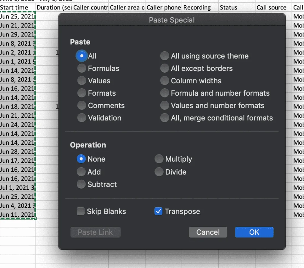
Simply select and copy the data you want to transform into columns, select Paste Special, check the Transpose option and press OK.

Your rows will become columns, and your columns will magically become rows – all in a few clicks.
Secret #4: Selecting datasets
Are you clicking and dragging to select a group of data? There’s a faster way!
- Click in the first cell you want to select and hold down Ctrl+Shift
- Then use the down arrow to get all the data in the column below
- Or the up arrow to get all the data above
- Or the left or right arrow to get everything in the row in either direction
- Combine multiple directional arrow keys to select data across the columns and rows that surround the cell you first clicked
- Use Ctrl+Shift+* to select the whole dataset
Secret #5: Autofill and Flash Fill
Excel will sometimes smartly fill a column based on the pattern of data it sees in the first column.
For example, if you want to change how a phone number is formatted, simply start changing the phone number in the first row, and Excel should recognise the pattern and make a suggestion. Simply hit Enter or Return to accept the change it has suggested.
You may need to manually ask Excel to perform a Flash Fill by clicking the option under the Data tab.
If Flash Fill doesn’t immediately spot a pattern when you think it should or lacks accuracy, simply give it a few more examples to work with, and it should work it out. Secret #6: Work With Cells Across Sheets
Flash Fill and autofill work for a wide range of patterns across numbers, dates, names, and other predictable types of content.
Secret #6: Work with cells across different sheets
The 3D Sum function works when you have multiple sheets in a workbook that all have the same basic layout, for example, a quarterly financial statement. For example, in cell A3, you always have the amount for the same corresponding week over time.
On a new worksheet in the workbook, go to a cell and type a formula like =sum(‘M1:M12’!A3). This is a SUM formula that adds up the value that week for all the sheets that are titled M1 to M12 (so a full year). It looks at cell A3 in each of those twelve sheets. The result will be the sum of all 12 months.
Secret #7: Conditional formatting
If you have a hefty amount of data to interpret or just want people to have an instant understanding of what your spreadsheet says, then you could benefit from Conditional Formatting.
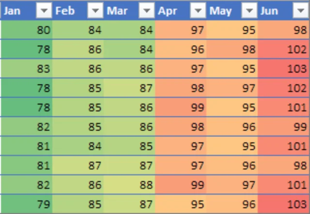
Excel’s Conditional Formatting will automatically change borders, background colours, and text styling based on the rules you set for your data.
For example, you could display a significant profit in bright green, closer to break-even in yellow, slight losses in orange, and significant losses in red. This will give you and anyone who sees your spreadsheet a clear at-a-glance understanding of the data.

Conditional Formatting can also build a graph into each cell so you can visualise the top and bottom of the range of numbers at a glance. You can even specify icons (known as ‘web dings’) to display to help add further meaning to your data and make it easier to interpret. What a great way to show off!

Look under Format for the Conditional Format option after selecting a dataset from your spreadsheet and then customise it to suit your needs.
Need a Microsoft 365 expert?
We help businesses and organisations throughout Scotland to meet their goals and grow their business using Excel and other essential tools featured in Microsoft 365 as part of our 365 cloud service.
Contact us today to begin the conversation about how we can help you utilise the full power of Microsoft 365 in your business while meeting your exact requirements and budget.


